
Embeddings are the cornerstone of any retrieval system. And the larger the embeddings, the more information they can store. But large embeddings require a lot of memory, which leads to high computational costs and latency. To reduce this high cost, we can use models that produce embeddings with sm
Embeddings are the cornerstone of any retrieval system. And the larger the embeddings, the more information they can store.
But large embeddings require a lot of memory, which leads to high computational costs and latency.
To reduce this high cost, we can use models that produce embeddings with small dimensions, but even that has a bunch of drawbacks. Smaller embeddings usually can't encapsulate as much semantic information as their larger counterparts.
For example, bert-base-uncased with 768 dimensions is not as good as OpenAI's text-embedding-3-large with 3072 dimensions.
Thus, we needed a solution that balances this tradeoff between latency/cost and semantic capture, and that is exactly what Matryoshka Representation Learning does.
This article will break down MRL, show you how to implement it, and how it has helped us at Supermemory build our memory engine.
What is Matryoshka Representation Learning (MRL)?
Matryoshka Representation Learning is a novel technique used to create vector embeddings with the same model, but with varying sizes.
Let's elaborate.
Usually, to create embeddings, we pass text through a model, and we get an embedding of a specific dimension, like 1024. Once you create this embedding, you can't change its dimensions.
But, in MRL, when we create an embedding, we can create embeddings of various sizes, like 128, 256, 768, etc. Creating smaller embeddings cuts compute and latency, which makes retrieval faster.
With Matryoshka Representation Learning, we do not train separate models for each dimension. We produce a single full vector and structure it so we can slice it to different sizes. Early dimensions carry the core semantics; later dimensions add finer detail.
This lets us run shortlisting and reranking efficiently: shortlist with a small prefix, then rerank with a larger slice for accuracy. We’ll dig into shortlisting and reranking next.
Shortlisting and Reranking
As the name suggests, this method is broken down into two main parts. The first one is:
- Shortlisting:
- Shortlisting is the process of using small-sized embeddings to retrieve a few top relevant documents very quickly.
- For example, retrieving 200 relevant documents from 1000 documents.
- Here, we trade off accuracy for speed and efficiency.
- Reranking:
- Here, we use full-sized embeddings to rerank the existing 200 documents.
- For example, D1, D2, D3 can become D2, D3, D1 after reranking.
- Reranking does not affect our efficiency, as we only perform it on a small number of documents compared to the original number of documents.
So, in short:
- First we use MRL to create varying embeddings.
- Then, we use smaller embeddings to retrieve a few top documents related to the query over a large set of documents.
- After that, we rerank or rearrange the retrieved documents.
Thus, we get the most relevant and important documents for the query.
How does MRL work?
MRL can create embeddings with varying dimensions. But, how exactly?
MRL is not an embedding model with a specific structure or something, but it's a method that can be applied to train any existing embedding model. It can even be used to fine-tune pre-trained models.
Given is the visual representation of how MRL can be applied over any existing embedding strategy:
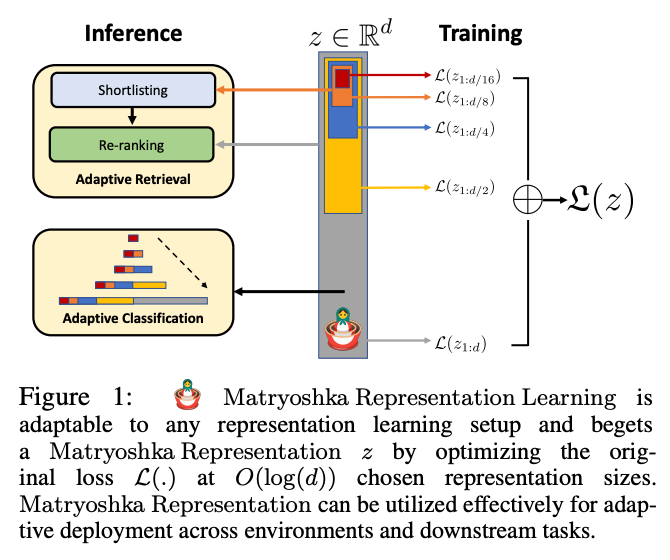
Before diving into the math and nitty-gritty of MRL, let's understand the core idea of MRL, which is calculating loss in a bit of a different way.
In MRL, you calculate a loss function for various dimensions instead of just one loss function for one fixed dimension size. Then, you add up or take the average of all the loss functions.
For instance, in a normal embedding model, we would calculate a single loss for a specific dimension like 1024.
But when it comes to MRL, we calculate loss for the original (larger) size of the embedding, but along with it, we also calculate loss for a list of dimensions (the values of these dimensions are a hyper-parameter and are fixed during training) like 128, 256, 764, and 1024.
Once we calculate this loss for each dimension, we then add/average them to get the final single loss value on which we will perform backpropagation to learn embeddings.
The Math Behind MRL
Except for the loss, all other processes in MRL are similar to any other embedding models.
Given is the loss function used by MRL:
$$
L_{\text{MRL}} = \sum_{m \in M} c_m \cdot L(z_{1:m})
$$
- \\(L_{\text{MRL}}\\) is the total Matryoshka loss.
- \\(M\\) is the set of pre-defined dimensions you want to train on (e.g.,
{64, 128, 256, 768}). - \\(m\\) is a specific dimension from the set M.
- $c_{m}$ is a weighting factor (relative importance) for the loss at dimension m. This is often set to 1 for all dimensions, giving them equal importance.
- $L$ is your base loss function (e.g., Cross-Entropy, Contrastive Loss).
- $z_{1:m}$ is the embedding vector truncated to its first m dimensions.
The weighting factor is used to give importance to a specific dimension size. Usually, it's set at 1 so that we give equal importance to all the dimensions and the model can learn a better representation at all dimension levels.
But for specific tasks, for instance extremely fast retrieval and low accuracy, we can use a weighting factor to give smaller dimension sizes more importance.
For example: $c_{128}=2.0$, $c_{256}=1.0$, $c_{768}=0.5$
A simpler formula for intuition:
$$
Loss = loss_{32} + loss_{64} + loss_{128} + loss_{256} + loss_{1024}
$$
A complex formula for no reason (given in the original research paper):
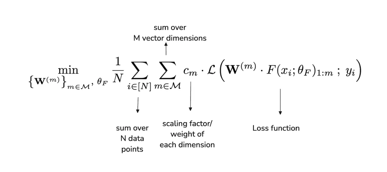
Standard Way vs. Matryoshka Way of Training
Standard Embedding Training
- Take input data (e.g., a sentence).
- Pass it through the model to get a single, full-sized embedding (e.g., 768 dimensions).
- Calculate one loss value based on how well that 768-dim embedding performs on the task (e.g., a contrastive loss in Sentence Transformers).
- The optimizer updates the model's weights based on that single loss.
Matryoshka Representation Learning (MRL) Training
- Take input data.
- Pass it through the model to get the single, full-sized embedding.
- Calculate multiple losses in parallel:
- Loss 1: On the full embedding (
vector[:]). - Loss 2: On a truncated prefix of the embedding (
vector[:512]). - Loss 3: On an even shorter prefix (
vector[:256]). - Loss 4: On the shortest prefix (
vector[:64]).
- Loss 1: On the full embedding (
- These individual loss values are then aggregated (e.g., summed or averaged) into a single, final loss value.
- The optimizer updates the model's weights based on this single aggregated loss.
Important, interesting notes
So, why the name 'Matryoshka'?
The name comes from Russian Matryoshka dolls, where smaller dolls are nested inside larger ones.
MRL works the same way with embeddings:
- The 128-dimension embedding is not just a separate, smaller embedding; it's literally the first 128 values of the larger 256-dimension embedding.
- The 256-dimension embedding is the first 256 values of the 768-dimension one, and so on.

MRL creates an embedding in such a way that our first few dimensions hold the semantic information with the highest value, i.e., they can explain the main idea or theme behind the text, or they encapsulate the most information about the text. The latter dimensions enrich that information with finer details.
Code Implementation
Let's look at the code of how we can implement MRL using the pre-trained MPnet base model,
import torch
from sentence_transformers import SentenceTransformer, util

model_name = 'tomaarsen/mpnet-base-nli-matryoshka'
model = SentenceTransformer(model_name)

source_sentence = "A person is riding a motorcycle on a road."
similar_sentence = "A man is on a motorbike on a street."
dissimilar_sentence = "The cat is sleeping on the kitchen table."

sentences = [source_sentence, similar_sentence, dissimilar_sentence]

full_embeddings = model.encode(sentences, convert_to_tensor=True)

matryoshka_dims = [64, 128, 256, 512, 768] # these are the different embeddings for which loss will be calculated and aggregated.

print(f"--- Using Model: '{model_name}' ---")
print(f"Full embedding dimension: {full_embeddings.shape[1]}")

for dim in matryoshka_dims:
	print(f"\n--- Testing with dimension: {dim} ---")

	sub_embeddings = full_embeddings[:, :dim]

	scores = util.cos_sim(sub_embeddings[0], sub_embeddings[1:])

	score_similar = scores[0][0]
	score_dissimilar = scores[0][1]

	print(f"Similarity with '{similar_sentence}': {score_similar.item():.4f}")
	print(f"Similarity with '{dissimilar_sentence}':{score_dissimilar.item():.4f}")
Output:
--- Using Model: 'tomaarsen/mpnet-base-nli-matryoshka' ---
Full embedding dimension: 768

--- Testing with dimension: 64 ---
Similarity with 'A man is on a motorbike on a street.': 0.7775
Similarity with 'The cat is sleeping on the kitchen table.': -0.0945

--- Testing with dimension: 128 ---
Similarity with 'A man is on a motorbike on a street.': 0.7687
Similarity with 'The cat is sleeping on the kitchen table.': -0.0744

--- Testing with dimension: 256 ---
Similarity with 'A man is on a motorbike on a street.': 0.7727
Similarity with 'The cat is sleeping on the kitchen table.': -0.0648

--- Testing with dimension: 512 ---
Similarity with 'A man is on a motorbike on a street.': 0.7630
Similarity with 'The cat is sleeping on the kitchen table.': -0.0106

--- Testing with dimension: 768 ---
Similarity with 'A man is on a motorbike on a street.': 0.7516
Similarity with 'The cat is sleeping on the kitchen table.': 0.0294
Here we initialize MPnet base model using the SentenceTransformer() library. Then we create a source sentence and two more example sentences, such that one is similar to the source and the other is dissimilar.
The motive behind creating these two sentences is to check the similarity of the source with both of them. We compute the similarity score for all the Matryoshka dimensions. Sentences are then embedded using an embedding model (one which is specifically trained with the Matryoshka loss method).
We use a for loop to iterate over all the dimensions in matryoshka_dims, and for each dimension, we slice the full embedding into a smaller size (same as the dimension).
These smaller embeddings are then used to calculate the similarity score between the source sentence and the example sentences (both similar and dissimilar ones) using Cosine Similarity.
In the end, we print the similarity scores for each embedding dimension so that we can compare how each embedding performs.
How we use MRL at Supermemory and our learnings
We started with full-length provider embeddings, around 3k dims in our case, and hit the usual pain points: big indexes, slower queries, and rising storage.
After reading Exa’s write-up on billion-scale storage, we tried Matryoshka-style embeddings and kept them in production.
What we do uniquely, which I think a lot of other people don't know is, not just slicing, but also normalization of the embeddings and quantizing them.
Normalization
Prefix slices live in a smaller subspace. If you use them raw, vectors spread out more than they should and cosine scores get jumpy. We L2-normalize embeddings so that a 64-, 128-, or 256-dim slice sits in a stable geometry.
We compute the sum of squares, take the square root, and divide the vector by that norm. We apply the same idea to prefixes, so a 128-dim slice is scaled in proportion to the part of the space we are using.
This simple step tightened precision and pulled in items that were previously missed. It also increased separation where it mattered, pushing clearly unrelated pairs further apart.
Quantization.
After normalization, we apply lightweight quantization. Storage drops a lot without a noticeable quality hit for our workload. We still keep the full embedding, and we also keep a compact view for fast paths.
Storage goes up a bit overall, but index size and query speed improve where it counts.
Quality vs dimension.
Empirically, halving the dimension kept quality near intact for us, and going down to roughly one third still preserved most of it. That let us shortlist on small prefixes and reserve the full vector for rerank.
Provider tips.
If the API lets you request a target dimension, ask for it directly. Smaller outputs come back faster. Some providers also return those smaller vectors pre-normalized. In our tests, Voyage does; Google does not.
The main tradeoff is that slicing can lose certain latent interactions that only exist in the full space.
That tradeoff is worth it in practice for us, and it is one reason our memory lookups are fast in production, with end-to-end retrieval and rerank routinely under 200 ms.
If you want to add real memory instead of a vector dump to your LLMs and agents, try Supermemory with your data and see the difference in recall and response quality.
Get started in just 5 mins.


